Update (13-12-2013) Hakka Labs, who kindly recorded my talk at the NYC Machine Learning meetup, have put the video and slides online.
My Ph.D., which I completed earlier this year, was about outlier selection and one-class classification. During this time I learned about quite a few machine learning algorithms; especially about outlier-selection algorithms and one-class classifiers, of course. With some help of Ferenc Huszár and Laurens van der Maaten, I also came up with a new outlier-selection algorithm called Stochastic Outlier Selection (SOS), which I would like to briefly describe here.
If you prefer a more detailed discussion about the algorithm, the experiments, and the results, you can read either the technical report (PDF) or chapter 4 of my Ph.D. thesis. In case you can’t wait to see whether your own dataset contains any outliers then there’s a Python implementation of SOS which you can also use from the command-line.
Affinity-based outlier selection
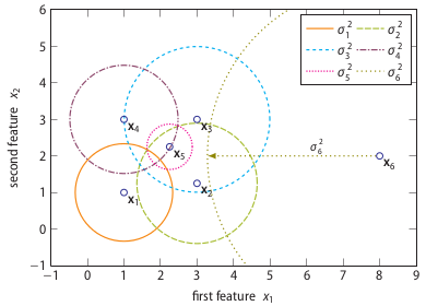
SOS is an unsupervised outlier-selection algorithm that takes as input either a feature matrix or a dissimilarity matrix and outputs for each data point an outlier probability. Intuitively, a data point is considered to be an outlier when the other data points have insufficient affinity with it. Allow me to explain this using the following two-dimensional toy dataset.
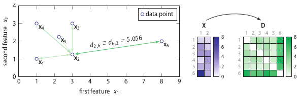
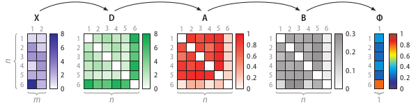
The right part of the figure shows that the feature matrix X is transformed into a dissimilarity matrix D using the Euclidean distance. (Any dissimilarity measure could have been used here.) Using the dissimilarity matrix D, SOS computes an affinity matrix A, a binding probability matrix B, and finally, the outlier probability vector Φ, because Greek letters are cool.
The use of the concept of affinity is inspired by t-Distributed Stochastic Neighbor Embedding (t-SNE), which is a non-linear dimensionality reduction technique created by Laurens van der Maaten and Geoffrey Hinton. Both algorithms use the concept of affinity to quantify the relationship between data points. t-SNE uses it to preserve the local structure of a high-dimensional dataset and SOS uses it to select outliers. The affinity a certain data point has with another data point decreases Gaussian-like with respect to their dissimilarity.
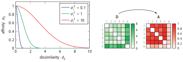
Each data point has a variance associated with it. The variance depends on the density of the neighborhood. A higher density implies a lower variance. In fact, the variance is set such that each data point has effectively the same number of neighbors. This number is controlled via the only parameter of SOS, called perplexity.
Perplexity can be interpreted as the k in k-nearest neighbor algorithms. The difference is that in SOS being a neighbor is not a binary property, but a probabilistic one. The following figure illustrates the binding probabilities data point x1 (or vertex v1 because we have switched to a graph representation of the dataset) has with the other five data points.
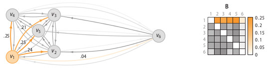
The binding probability matrix is just the affinity matrix such that the rows sum to 1. To obtain the outlier probability of data point we compute the joint probability that the other data points will not bind to it.
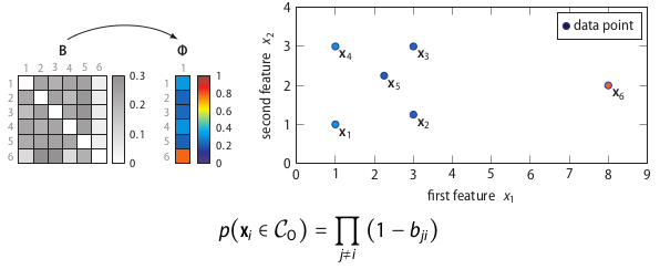
This simple equation corresponds to the intuition behind SOS mentioned earlier: a data point is considered to be an outlier when the other data points have insufficient affinity with it. The proof behind this equation is unfortunately beyond the scope of this post.
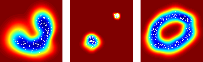
SOS has been evaluated on a variety of real-world and synthetic datasets, and compared to four other outlier-selection algorithms. The following figure shows the weighted AUC performance on 18 real-world datasets.
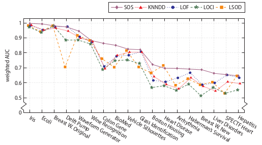
As you can see, SOS has a higher performance on most of these real-world datasets. However, there’s still the no-free-lunch theorem, which basically says that no algorithm uniformly outperforms all other algorithms on all datasets. So, if you’d like to select some outliers on your own dataset, check out SOS by all means, but keep in mind that you may obtain a higher performance with a different outlier-selection algorithm. The real questions are: which one and why?
As this was a very brief description of SOS, I had to skip over many details. Again, in case you’re interested, you can read either the technical report (PDF) or chapter 4 of my Ph.D. thesis. In the next section I apply SOS to roll call voting data.
Detecting anomalous senators
Last week, I had the pleasure to talk about outlier selection and one-class classification at the NYC Machine Learning meetup. Hakka Labs recorded it, and put the video and slides online. In order to not just show fancy graphs and boring equations I created a demo in D3 and CoffeeScript, of which you see a screenshot below. In the demo, I apply SOS on roll call voting data, which is inspired by this post on visualizing the senate by Vik Paruchuri. The demo illustrates how the approximated outlier probability of each senator evolves as more Stochastic Neighbor Graphs (SNG) are being sampled. (Please note that SNGs are not discussed in this post.)
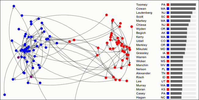
Let’s see how the approximated outlier probabilities compare to the outlier probabilities computed on the command-line. Recently, I started using drake to organize my data workflow. (If you care about reproducibility, then I recommend you try it out.) The following Drakefile shows how to fetch the roll call voting data, extract its features and labels, and apply the Python implementation of SOS with a perplexity of 50 to it.
cat Drakefile

;# Get dataset
dataset.csv <- [-timecheck]
	curl -s https://raw.github.com/VikParuchuri/political-positions/master/113_frame.csv > $OUTPUT

;# Extract features
features.csv <- dataset.csv
	csvcut $INPUT -C 1,name,party,state | sed '1d;s/NA/4/g' > $OUTPUT

;# Extract labels
labels.csv <- dataset.csv
	csvcut $INPUT -c name,party,state > $OUTPUT

;# Compute outlier probabilities using SOS
outlier.csv <- features.csv
	echo 'outlier' > $OUTPUT
	< $INPUT sos -p 50 >> $OUTPUT

;# Combine labels and outlier probabilities and sort
result.csv <- labels.csv, outlier.csv
	paste -d, $INPUT0 $INPUT1 | csvsort -rc outlier > $OUTPUT
drake
head result.csv | csvlook

|-------------+-------+-------+-------------|
|  name       | party | state | outlier     |
|-------------+-------+-------+-------------|
|  Cowan      | D     | MA    | 0.91758412  |
|  Lautenberg | D     | NJ    | 0.89442425  |
|  Chiesa     | R     | NJ    | 0.8457114   |
|  Markey     | D     | MA    | 0.7813504   |
|  Kerry      | D     | MA    | 0.75302407  |
|  Wyden      | D     | OR    | 0.70110306  |
|  Murkowski  | R     | AK    | 0.68868458  |
|  Alexander  | R     | TN    | 0.626972    |
|  Vitter     | R     | LA    | 0.59739462  |
|-------------+-------+-------+-------------|
The tools csvcut, csvsort, and csvlook are part of csvkit.
You may notice that the outlier probabilities shown in the screenshot do not match the exact ones computed with sos. That’s because (1) the screenshot was taken not long after the demo started and (2) the demo was running in Chrome, which apparently has a different implementation of Math.random. In Firefox, the approximated outlier probabilities will match the exact ones, eventually.
If you enjoyed this post then you may want to follow me on Twitter.