Colors

One of raylibr’s nicest features is that R’s 657 built-in color names work everywhere a color is expected. This guide covers the full color system.

R color names

Any function that takes a color argument accepts an R color name as a string:

colors <- c(
  "tomato", "orangered", "gold", "yellow",
  "mediumseagreen", "seagreen", "steelblue", "dodgerblue",
  "slateblue", "mediumpurple", "orchid", "hotpink",
  "salmon", "coral", "khaki", "palegreen",
  "skyblue", "plum", "sienna", "grey70"
)

raylibr_screenshot(function() {
  cols <- 5L
  w <- 70L
  h <- 50L
  pad <- 10L
  for (i in seq_along(colors)) {
    row <- (i - 1L) %/% cols
    col <- (i - 1L) %% cols
    x <- pad + col * (w + pad)
    y <- pad + row * (h + pad + 14L)
    draw_rectangle(as.integer(x), as.integer(y), w, h, colors[i])
    draw_text(colors[i], as.integer(x + 2L), as.integer(y + h + 1L), 10L, "grey70")
  }
})

raylibr image

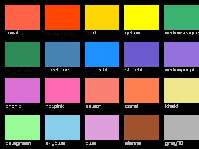
This includes all of colors() from base R — "red", "steelblue", "grey90", "antiquewhite", and 653 more.

The color struct

For precise control, construct colors with RGBA values (0–255):

col <- color(255, 100, 50, 255)
col$r
#> [1] 255
col$a
#> [1] 255

Convert from other representations with as_color():

as_color("tomato")
#> color(r = 255, g = 99, b = 71, a = 255)
as_color(0xFF6347FF)
#> color(r = 255, g = 99, b = 71, a = 255)

Transparency

color_alpha() creates a transparent version of any color. The alpha ranges from 0 (invisible) to 1 (opaque):

raylibr_screenshot(function() {
  draw_circle(150L, 130L, 80.0, "tomato")
  draw_circle(200L, 130L, 80.0, color_alpha("steelblue", 0.6))
  draw_circle(250L, 130L, 80.0, color_alpha("gold", 0.6))
  draw_circle(175L, 180L, 80.0, color_alpha("mediumseagreen", 0.5))
  draw_circle(225L, 180L, 80.0, color_alpha("orchid", 0.5))
})

raylibr image

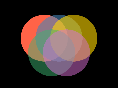
fade() does the same thing as color_alpha() — both set the alpha channel.

Color manipulation

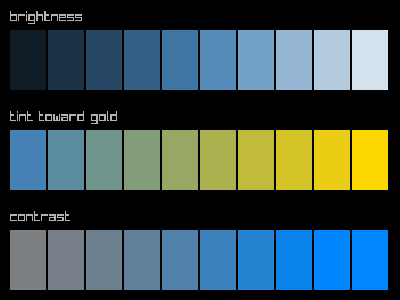
raylibr provides functions to adjust colors:

raylibr_screenshot(function() {
  base <- "steelblue"
  w <- 36L
  h <- 60L

  # Brightness: -255 to 255
  draw_text("brightness", 10L, 10L, 14L, "grey70")
  for (i in 0:9) {
    b <- -200 + i * 44
    draw_rectangle(10L + as.integer(i) * (w + 2L), 30L, w, h,
                   color_brightness(base, b / 255))
  }

  # Tint
  draw_text("tint toward gold", 10L, 110L, 14L, "grey70")
  for (i in 0:9) {
    frac <- i / 9
    draw_rectangle(10L + as.integer(i) * (w + 2L), 130L, w, h,
                   color_lerp(base, "gold", frac))
  }

  # Contrast: -255 to 255
  draw_text("contrast", 10L, 210L, 14L, "grey70")
  for (i in 0:9) {
    c_val <- -200 + i * 44
    draw_rectangle(10L + as.integer(i) * (w + 2L), 230L, w, h,
                   color_contrast(base, c_val / 255))
  }
})

raylibr image

• color_brightness(color, factor) — lighten (positive) or darken (negative)
• color_contrast(color, factor) — increase or decrease contrast
• color_tint(color, tint) — tint a color toward another

HSV color space

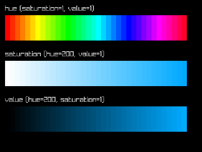
color_from_hsv() creates colors from hue (0–360), saturation (0–1), and value (0–1). This is great for generating color ramps:

raylibr_screenshot(function() {
  n <- 36L
  w <- as.integer(380 / n)
  # Hue rainbow
  draw_text("hue (saturation=1, value=1)", 10L, 10L, 14L, "grey70")
  for (i in 0:(n - 1L)) {
    draw_rectangle(10L + as.integer(i) * w, 30L, w, 50L,
                   color_from_hsv(i * 360.0 / n, 1.0, 1.0))
  }
  # Saturation ramp
  draw_text("saturation (hue=200, value=1)", 10L, 100L, 14L, "grey70")
  for (i in 0:(n - 1L)) {
    draw_rectangle(10L + as.integer(i) * w, 120L, w, 50L,
                   color_from_hsv(200.0, i / (n - 1.0), 1.0))
  }
  # Value ramp
  draw_text("value (hue=200, saturation=1)", 10L, 190L, 14L, "grey70")
  for (i in 0:(n - 1L)) {
    draw_rectangle(10L + as.integer(i) * w, 210L, w, 50L,
                   color_from_hsv(200.0, 1.0, i / (n - 1.0)))
  }
})

raylibr image

Convert back with color_to_hsv():

color_to_hsv("tomato")
#>         x         y         z 
#> 9.1304340 0.7215686 1.0000000

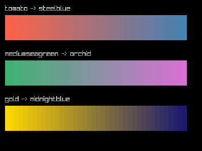
Interpolation

color_lerp() blends between two colors. Use it to create smooth gradients:

raylibr_screenshot(function() {
  n <- 40L
  w <- as.integer(380 / n)

  from <- "tomato"
  to <- "steelblue"
  draw_text("tomato -> steelblue", 10L, 10L, 14L, "grey70")
  for (i in 0:(n - 1L)) {
    draw_rectangle(10L + as.integer(i) * w, 30L, w, 50L,
                   color_lerp(from, to, i / (n - 1.0)))
  }

  from2 <- "mediumseagreen"
  to2 <- "orchid"
  draw_text("mediumseagreen -> orchid", 10L, 100L, 14L, "grey70")
  for (i in 0:(n - 1L)) {
    draw_rectangle(10L + as.integer(i) * w, 120L, w, 50L,
                   color_lerp(from2, to2, i / (n - 1.0)))
  }

  from3 <- "gold"
  to3 <- "midnightblue"
  draw_text("gold -> midnightblue", 10L, 190L, 14L, "grey70")
  for (i in 0:(n - 1L)) {
    draw_rectangle(10L + as.integer(i) * w, 210L, w, 50L,
                   color_lerp(from3, to3, i / (n - 1.0)))
  }
})

raylibr image

color_alpha_blend() blends a foreground color over a background, respecting the foreground’s alpha channel — useful for compositing.